6.3.1. Confounds exploration

Here we show how to regress out confound signals, in particular using statistical CompCor.

• Y. Behzadi et al. A Component Based Noise Correction Method (CompCor) for BOLD and Perfusion Based fMRI, NeuroImage Vol 37 (2007), p. 90-101

6.3.1.1. Statistical CompCor

Retrieve the data from one subject

from sammba import data_fetchers

test_retest = data_fetchers.fetch_zurich_test_retest(subjects=[1])
fmri_filename = test_retest.func[0]

We perform a PCA to extract the 98% most variant components. This is done by the function nilearn.image.high_variance_confounds,

from nilearn import image

hv_array = image.high_variance_confounds(fmri_filename)
print('Computed {0} confounds array.'.format(hv_array.shape[1]))

Out:

Computed 5 confounds array.

6.3.1.2. Do my counfounds model noise properly? Voxel-to-voxel connectivity tells!

Check the relevance of chosen confounds: The distribution of voxel-to-voxel correlations should be tight and approximately centered to zero.

Compute voxel-wise time series without confounds removal, using NiftiMasker.

from nilearn.input_data import NiftiMasker

brain_masker = NiftiMasker(detrend=True, memory='nilearn_cache', verbose=1)
timeseries_raw = brain_masker.fit_transform(fmri_filename)

Out:

[NiftiMasker.fit] Loading data from /home/salma/nilearn_data/zurich_retest/baseline/1367/rsfMRI.nii.gz
[NiftiMasker.fit] Computing the mask
[NiftiMasker.fit] Resampling mask

Next, compute the voxel-to-voxel correlations. We use only 1% of voxels, to save computation time.

import numpy as np

selected_voxels = range(0, timeseries_raw.shape[1], 100)
correlations_raw = np.corrcoef(timeseries_raw[:, selected_voxels].T)

Same thing, with counfounds removed: compute voxelwise time-series

timeseries_cleaned = brain_masker.fit_transform(
    fmri_filename, confounds=[hv_array])
correlations_cleaned = np.corrcoef(timeseries_cleaned[:, selected_voxels].T)

Out:

[NiftiMasker.fit] Loading data from /home/salma/nilearn_data/zurich_retest/baseline/1367/rsfMRI.nii.gz
[NiftiMasker.fit] Computing the mask
[NiftiMasker.fit] Resampling mask

Plot now the histograms of both raw and cleaned correlations.

import matplotlib.pylab as plt

plt.figure(figsize=(8, 5))
plt.hist(correlations_raw[np.triu_indices_from(correlations_raw, k=1)],
         color='r', alpha=.3, bins=100, lw=0, label='raw')
plt.hist(correlations_cleaned[np.triu_indices_from(correlations_cleaned, k=1)],
         color='b', alpha=.3, bins=100, lw=0, label='cleaned')

[ymin, ymax] = plt.ylim()
plt.vlines(0, ymin, ymax)
plt.xlabel('correlation values')
plt.title('voxel-to-voxel correlations')
plt.legend()
plt.tight_layout()
plt.show()

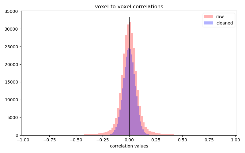
The correlations distribution is wider after statistical CompCor, so these confounds are not well suited to our case.

Total running time of the script: ( 0 minutes 2.495 seconds)